Sunlight beam progression over a few weeks
This post was originally published on my old blog dedicated to amateur astronomy.
Recently I was working at my office when I noticed a light beam that wasn’t there on the previous days. I knew it was going to get bigger during the next days, so I decided to record it for a few weeks, plot a chart and make some calculations out of it, just for fun.
In total 14 days were recorded, but not in a 14-day time span. The first picture was taken August 20th and the last on September 12th. The missing pictures relates to days in which the weather was blocking the beam to be visible.
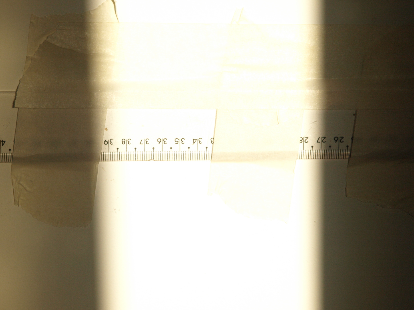
I used a fixed metric ruler on the wall and took a picture every day roughly at the same time (4:30pm).
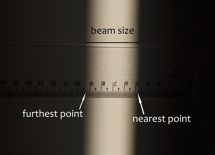
It changed every day. Not only the beam size was getting bigger but the “furthest” and “nearest” point were both moving to the left. This chart plots the evolution:
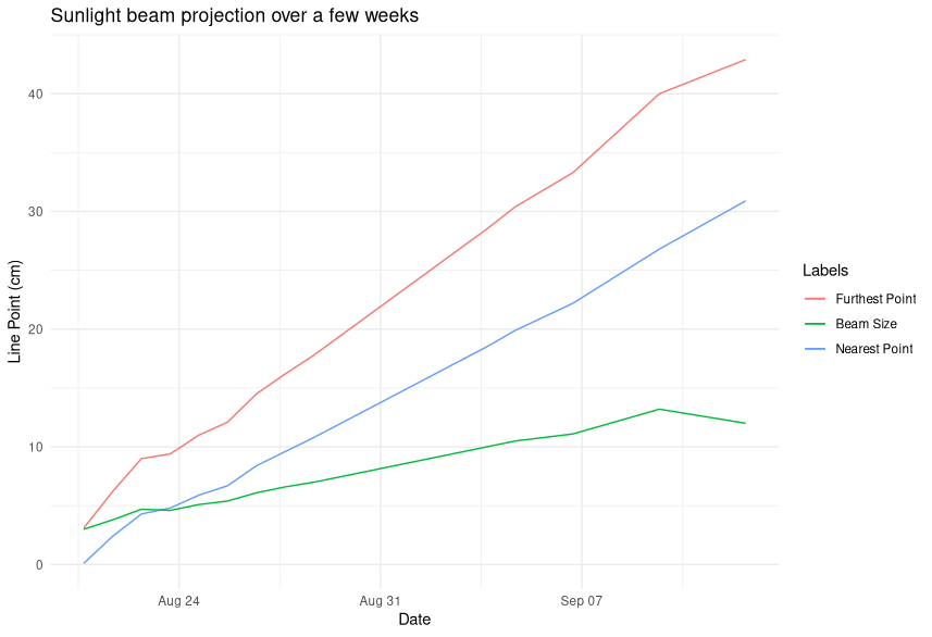
That’s the CSV data I created for this chart:
id,file,taken_at,starts,ends
1,P8204296.jpg,2020-08-20T16:29,0.1,3.1
2,P8214342.jpg,2020-08-21T16:33,2.4,6.2
3,P8224394.jpg,2020-08-22T16:37,4.3,9
4,P8234409.jpg,2020-08-23T16:33,4.8,9.4
5,P8244481.jpg,2020-08-24T16:33,5.9,11
6,P8254490.jpg,2020-08-25T16:31,6.7,12.1
7,P8264510.jpg,2020-08-26T16:33,8.4,14.5
8,P8274534.jpg,2020-08-27T16:34,9.6,16.2
9,P8284562.jpg,2020-08-28T16:33,10.8,17.8
10,P9034712.jpg,2020-09-03T16:33,18.5,28.5
11,P9044761.jpg,2020-09-04T16:33,19.9,30.4
12,P9064818.jpg,2020-09-06T16:31,22.2,33.3
13,P9094866.jpg,2020-09-09T16:34,26.8,40,0
14,P9124956.jpg,2020-09-12T16:34,30.9,42.9
And that’s the R script I wrote to plot it:
sunlight.data <- read.csv(file="~/sunlight_experiment.csv")
sunlight.data$taken_at <- as.POSIXct(sunlight.data$taken_at, format = "%Y-%m-%dT%H:%M", tz = "America/Maceio")
sunlight.data$size <- (sunlight.data$ends - sunlight.data$starts)

ggplot(sunlight.data, aes(x=taken_at)) +
  labs(title = "Sunlight beam projection over a few weeks") +
  geom_line(aes(y = starts, color = "darkred")) +
  geom_line(aes(y = ends, color = "darkblue")) +
  geom_line(aes(y = size, color = "darkgreen")) +
  scale_color_discrete(name = "Labels", labels = c("Furthest Point", "Beam Size", "Nearest Point")) +
  xlab("Date") +
  ylab("Line Point (cm)")
I also wrote a super simple Elixir program to compute the growth average for these values:
defmodule SunLightExperiment do
  @moduledoc false

  alias Decimal, as: D
  require Logger

  @doc false
  def perform do
    with data <- read_data("data.csv"),
         starts_growth <- compute_growth(data, :starts),
         ends_growth <- compute_growth(data, :ends),
         size_growth <- compute_growth(data, :size),
         starts_growth_average <- average(starts_growth),
         ends_growth_average <- average(ends_growth),
         size_growth_average <- average(size_growth) do
      Logger.info("Printing results...")

      IO.inspect(data)
      IO.puts("\n'starts' growth: #{inspect(starts_growth)}\n")
      IO.puts("'ends' growth: #{inspect(ends_growth)}\n")
      IO.puts("'size' growth: #{inspect(size_growth)}\n")
      IO.puts("'starts' growth average: #{inspect(starts_growth_average)}\n")
      IO.puts("'ends' growth average: #{inspect(ends_growth_average)}\n")
      IO.puts("'size' growth average: #{inspect(size_growth_average)}")
    end
  end

  @spec read_data(String.t()) :: Enumerable.t()
  defp read_data(file) do
    file
    |> File.stream!()
    |> CSV.decode()
    |> Stream.take(10)
    |> Stream.map(&get_valid_row/1)
    |> Stream.drop(1)
    |> Stream.map(&trim_columns/1)
    |> Stream.map(&to_entry/1)
    |> Enum.filter(fn entry -> entry != %{} end)
  end

  @spec compute_growth(list(map()), atom()) :: list(D.t())
  defp compute_growth(results, v) do
    Enum.reduce(results, [], fn result, acc ->
      case result == Enum.at(results, 0) do
        true ->
          acc

        _any ->
          acc ++ [D.sub(Map.get(result, v), tnm1(results, v, Enum.count(acc) + 1))]
      end
    end)
  end

  @spec average(list(D.t())) :: D.t()
  defp average(list) do
    with count <- Enum.count(list),
         count <- D.new(count),
         sum <- Enum.reduce(list, D.new(0), fn e, acc -> D.add(e, acc) end) do
      D.div(sum, count)
    end
  end

  @spec tnm1(list(map()), atom(), integer()) :: D.t()
  defp tnm1(results, variable, n) do
    results
    |> Enum.at(n - 1)
    |> Map.get(variable)
  end

  @spec get_valid_row({:ok, list(String.t())} | any()) :: list(String.t())
  defp get_valid_row(result) do
    case result do
      {:ok, row} -> row
      _any -> []
    end
  end

  @spec to_entry(list(String.t())) :: {:ok, Entry.t()} | {:error, Error.t()}
  defp to_entry([id, filename, taken_at, starts, ends]) do
    with {:ok, taken_at, _offset} <- DateTime.from_iso8601(taken_at),
         {starts, _any} <- D.parse(starts),
         {ends, _any} <- D.parse(ends),
         entry <- do_to_entry(id, filename, taken_at, starts, ends) do
      entry
    end
  end

  defp to_entry(_any) do
    %{}
  end

  @spec do_to_entry(String.t(), String.t(), DateTime.t(), D.t(), D.t()) :: map()
  defp do_to_entry(id, filename, taken_at, starts, ends) do
    %{
      id: id,
      filename: filename,
      taken_at: taken_at,
      starts: starts,
      ends: ends,
      size: D.sub(ends, starts)
    }
  end

  @spec trim_columns(list(String.t())) :: list(String.t())
  defp trim_columns(row) do
    Enum.map(row, fn
      column when is_binary(column) -> String.trim(column)
      column -> column
    end)
  end
end
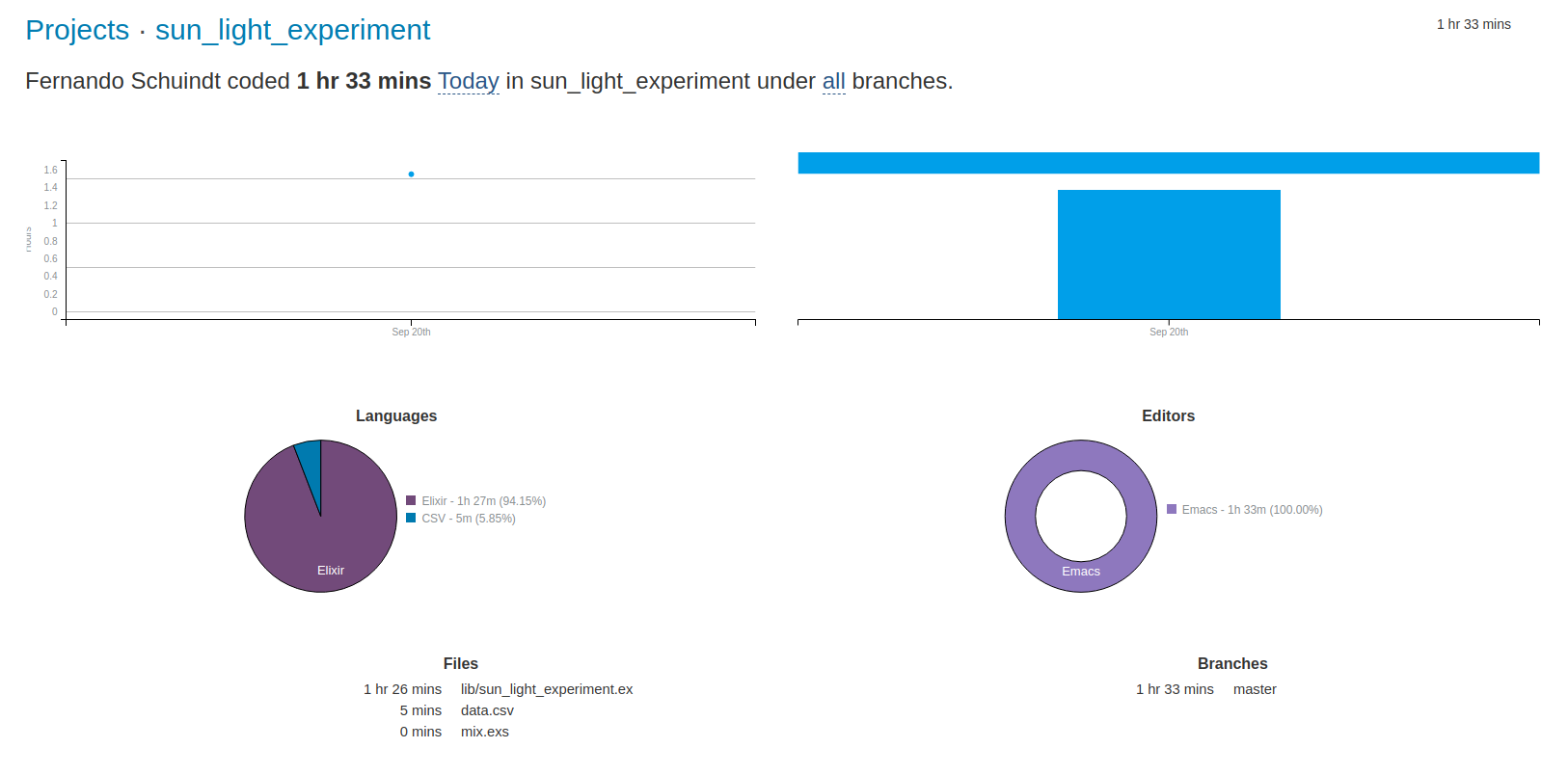
According to Wakatime I took 1 hour and 33 minutes to write this one:
And the results are:
- The “nearest point” moved to the left with a average speed of 1.34cm per day.
- The “furthest point” moved to the left with a average speed of 1.84cm per day.
- The “beam size” grew about 0.5cm per day.
I made the calculations using only the first 8 days, as they were separated with a almost precise 24h interval. This whole thing was a proof of concept for a later iteration of this experiment. The amount of data and the lack of precision yielded funky numbers, but this was expected in some sense. I think the overall outcome of this experiment is positive, I feel ready to start processing some more serious data.
And of course, that’s the beam on the first day, August 20th:
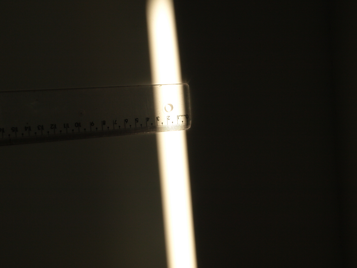
Now it on the last day, September 12th:
Click here to see all the images.